Chapter 3 Programming basics
We teach R because it greatly facilitates data analysis, the main topic of this book. By coding in R, we can efficiently perform exploratory data analysis, build data analysis pipelines, and prepare data visualization to communicate results. However, R is not just a data analysis environment but a programming language. Advanced R programmers can develop complex packages and even improve R itself, but we do not cover advanced programming in this book. Nonetheless, in this section, we introduce three key programming concepts: conditional expressions, for-loops, and functions. These are not just key building blocks for advanced programming, but are sometimes useful during data analysis. We also note that there are several functions that are widely used to program in R but that we will not cover in this book. These include split, cut, do.call, and Reduce, as well as the data.table package. These are worth learning if you plan to become an expert R programmer.
3.1 Conditional expressions
Conditional expressions are one of the basic features of programming. They are used for what is called flow control. The most common conditional expression is the if-else statement. In R, we can actually perform quite a bit of data analysis without conditionals. However, they do come up occasionally, and you will need them once you start writing your own functions and packages.
Here is a very simple example showing the general structure of an if-else statement. The basic idea is to print the reciprocal of a unless a is 0:
Let’s look at one more example using the US murders data frame:
Here is a very simple example that tells us which states, if any, have a murder rate lower than 0.5 per 100,000. The if-else statement protects us from the case in which no state satisfies the condition.
ind <- which.min(murder_rate)

if(murder_rate[ind] < 0.5){
  print(murders$state[ind])
} else{
  print("No state has murder rate that low")
}
#> [1] "Vermont"
If we try it again with a rate of 0.25, we get a different answer:
if(murder_rate[ind] < 0.25){
  print(murders$state[ind])
} else{
  print("No state has a murder rate that low.")
}
#> [1] "No state has a murder rate that low."
A related function that is very useful is ifelse. This function takes three arguments: a logical and two possible answers. If the logical is TRUE, the value in the second argument is returned and if FALSE, the value in the third argument is returned. Here is an example:
The function is particularly useful because it works on vectors. It examines each entry of the logical vector and returns elements from the vector provided in the second argument, if the entry is TRUE, or elements from the vector provided in the third argument, if the entry is FALSE.
| a | is_a_positive | answer1 | answer2 | result |
|---|---|---|---|---|
| 0 | FALSE | Inf | NA | NA |
| 1 | TRUE | 1.00 | NA | 1.0 |
| 2 | TRUE | 0.50 | NA | 0.5 |
| -4 | FALSE | -0.25 | NA | NA |
| 5 | TRUE | 0.20 | NA | 0.2 |
Here is an example of how this function can be readily used to replace all the missing values in a vector with zeros:
Two other useful functions are any and all. The any function takes a vector of logicals and returns TRUE if any of the entries is TRUE. The all function takes a vector of logicals and returns TRUE if all of the entries are TRUE. Here is an example:
3.2 Defining functions
As you become more experienced, you will find yourself needing to perform the same operations over and over. A simple example is computing averages. We can compute the average of a vector x using the sum and length functions: sum(x)/length(x). Because we do this repeatedly, it is much more efficient to write a function that performs this operation. This particular operation is so common that someone already wrote the mean function and it is included in base R. However, you will encounter situations in which the function does not already exist, so R permits you to write your own. A simple version of a function that computes the average can be defined like this:
Now avg is a function that computes the mean:
Notice that variables defined inside a function are not saved in the workspace. So while we use s and n when we call avg, the values are created and changed only during the call. Here is an illustrative example:
Note how s is still 3 after we call avg.
In general, functions are objects, so we assign them to variable names with <-. The function function tells R you are about to define a function. The general form of a function definition looks like this:
my_function <- function(VARIABLE_NAME){
  perform operations on VARIABLE_NAME and calculate VALUE
  VALUE
}
The functions you define can have multiple arguments as well as default values. For example, we can define a function that computes either the arithmetic or geometric average depending on a user defined variable like this:
We will learn more about how to create functions through experience as we face more complex tasks.
3.3 Namespaces
Once you start becoming more of an R expert user, you will likely need to load several add-on packages for some of your analysis. Once you start doing this, it is likely that two packages use the same name for two different functions. And often these functions do completely different things. In fact, you have already encountered this because both dplyr and the R-base stats package define a filter function. There are five other examples in dplyr. We know this because when we first load dplyr we see the following message:
The following objects are masked from ‘package:stats’:

    filter, lag

The following objects are masked from ‘package:base’:

    intersect, setdiff, setequal, union
So what does R do when we type filter? Does it use the dplyr function or the stats function? From our previous work we know it uses the dplyr one. But what if we want to use the stats version?
These functions live in different namespaces. R will follow a certain order when searching for a function in these namespaces. You can see the order by typing:
The first entry in this list is the global environment which includes all the objects you define.
So what if we want to use the stats filter instead of the dplyr filter but dplyr appears first in the search list? You can force the use of a specific namespace by using double colons (::) like this:
If we want to be absolutely sure that we use the dplyr filter, we can use
Also note that if we want to use a function in a package without loading the entire package, we can use the double colon as well.
For more on this more advanced topic we recommend the R packages book12.
3.4 For-loops
The formula for the sum of the series 1+2+⋯+n is n(n+1)/2. What if we weren’t sure that was the right function? How could we check? Using what we learned about functions we can create one that computes the Sn:
How can we compute Sn for various values of n, say n=1,…,25? Do we write 25 lines of code calling compute_s_n? No, that is what for-loops are for in programming. In this case, we are performing exactly the same task over and over, and the only thing that is changing is the value of n. For-loops let us define the range that our variable takes (in our example n=1,…,10), then change the value and evaluate expression as you loop.
Perhaps the simplest example of a for-loop is this useless piece of code:
Here is the for-loop we would write for our Sn example:
m <- 25
s_n <- vector(length = m) # create an empty vector
for(n in 1:m){
  s_n[n] <- compute_s_n(n)
}
In each iteration n=1, n=2, etc…, we compute Sn and store it in the nth entry of s_n.
Now we can create a plot to search for a pattern:
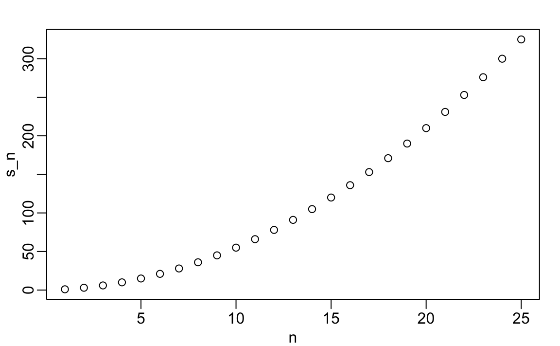
If you noticed that it appears to be a quadratic, you are on the right track because the formula is n(n+1)/2.
3.5 Vectorization and functionals
Although for-loops are an important concept to understand, in R we rarely use them. As you learn more R, you will realize that vectorization is preferred over for-loops since it results in shorter and clearer code. We already saw examples in the Vector Arithmetic section. A vectorized function is a function that will apply the same operation on each of the vectors.
x <- 1:10
sqrt(x)
#>  [1] 1.00 1.41 1.73 2.00 2.24 2.45 2.65 2.83 3.00 3.16
y <- 1:10
x*y
#>  [1]   1   4   9  16  25  36  49  64  81 100
To make this calculation, there is no need for for-loops. However, not all functions work this way. For instance, the function we just wrote, compute_s_n, does not work element-wise since it is expecting a scalar. This piece of code does not run the function on each entry of n:
Functionals are functions that help us apply the same function to each entry in a vector, matrix, data frame, or list. Here we cover the functional that operates on numeric, logical, and character vectors: sapply.
The function sapply permits us to perform element-wise operations on any function. Here is how it works:
Each element of x is passed on to the function sqrt and the result is returned. These results are concatenated. In this case, the result is a vector of the same length as the original x. This implies that the for-loop above can be written as follows:
Other functionals are apply, lapply, tapply, mapply, vapply, and replicate. We mostly use sapply, apply, and replicate in this book, but we recommend familiarizing yourselves with the others as they can be very useful.
3.6 Exercises
1. What will this conditional expression return?
2. Which of the following expressions is always FALSE when at least one entry of a logical vector x is TRUE?
all(x)any(x)any(!x)all(!x)
3. The function nchar tells you how many characters long a character vector is. Write a line of code that assigns to the object new_names the state abbreviation when the state name is longer than 8 characters.
4. Create a function sum_n that for any given value, say n, computes the sum of the integers from 1 to n (inclusive). Use the function to determine the sum of integers from 1 to 5,000.
5. Create a function altman_plot that takes two arguments, x and y, and plots the difference against the sum.
6. After running the code below, what is the value of x?
7. Write a function compute_s_n that for any given n computes the sum Sn=12+22+32+…n2. Report the value of the sum when n=10.
8. Define an empty numerical vector s_n of size 25 using s_n <- vector("numeric", 25) and store in the results of S1,S2,…S25 using a for-loop.
9. Repeat exercise 8, but this time use sapply.
10. Repeat exercise 8, but this time use map_dbl.
11. Plot Sn versus n. Use points defined by n=1,…,25.
12. Confirm that the formula for this sum is Sn=n(n+1)(2n+1)/6.