Chapter 32 Machine learning in practice
Now that we have learned several methods and explored them with illustrative examples, we are going to try them out on a real example: the MNIST digits.
We can load this data using the following dslabs package:
The dataset includes two components, a training set and test set:
Each of these components includes a matrix with features in the columns:
and vector with the classes as integers:
class(mnist$train$labels)
#> [1] "integer"
table(mnist$train$labels)
#>
#>    0    1    2    3    4    5    6    7    8    9
#> 5923 6742 5958 6131 5842 5421 5918 6265 5851 5949
Because we want this example to run on a small laptop and in less than one hour, we will consider a subset of the dataset. We will sample 10,000 random rows from the training set and 1,000 random rows from the test set:
set.seed(1990)
index <- sample(nrow(mnist$train$images), 10000)
x <- mnist$train$images[index,]
y <- factor(mnist$train$labels[index])

index <- sample(nrow(mnist$test$images), 1000)
x_test <- mnist$test$images[index,]
y_test <- factor(mnist$test$labels[index])
32.1 Preprocessing
In machine learning, we often transform predictors before running the machine algorithm. We also remove predictors that are clearly not useful. We call these steps preprocessing.
Examples of preprocessing include standardizing the predictors, taking the log transform of some predictors, removing predictors that are highly correlated with others, and removing predictors with very few non-unique values or close to zero variation. We show an example below.
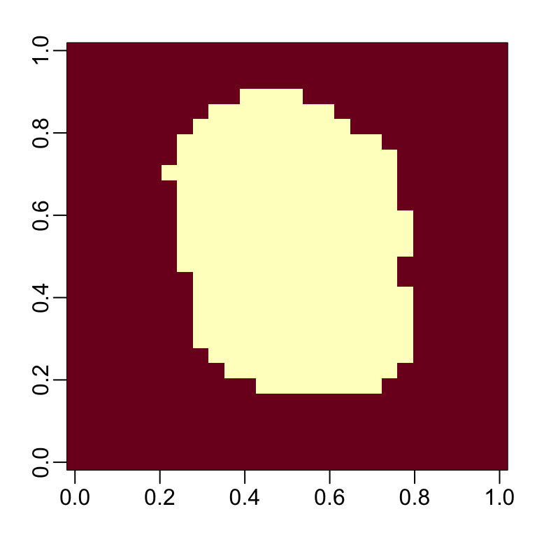
We can run the nearZero function from the caret package to see that several features do not vary much from observation to observation. We can see that there is a large number of features with 0 variability:
![]()
This is expected because there are parts of the image that rarely contain writing (dark pixels).
The caret packages includes a function that recommends features to be removed due to near zero variance:
We can see the columns recommended for removal:
So we end up keeping this number of columns:
Now we are ready to fit some models. Before we start, we need to add column names to the feature matrices as these are required by caret:
32.2 k-nearest neighbor and random forest
Let’s start with kNN. The first step is to optimize for \(k\). Keep in mind that when we run the algorithm, we will have to compute a distance between each observation in the test set and each observation in the training set. There are a lot of computations. We will therefore use k-fold cross validation to improve speed.
If we run the following code, the computing time on a standard laptop will be several minutes.
control <- trainControl(method = "cv", number = 10, p = .9)
train_knn <- train(x[ ,col_index], y,
                   method = "knn",
                   tuneGrid = data.frame(k = c(3,5,7)),
                   trControl = control)
train_knn
In general, it is a good idea to try a test run with a subset of the data to get an idea of timing before we start running code that might take hours to complete. We can do this as follows:
n <- 1000
b <- 2
index <- sample(nrow(x), n)
control <- trainControl(method = "cv", number = b, p = .9)
train_knn <- train(x[index, col_index], y[index],
                   method = "knn",
                   tuneGrid = data.frame(k = c(3,5,7)),
                   trControl = control)
We can then increase n and b and try to establish a pattern of how they affect computing time
to get an idea of how long the fitting process will take for larger values of n and b. You want to know if a function is going to take hours, or even days, before you run it.
Once we optimize our algorithm, we can fit it to the entire dataset:
We now achieve a high accuracy:
y_hat_knn <- predict(fit_knn, x_test[, col_index], type="class")
cm <- confusionMatrix(y_hat_knn, factor(y_test))
cm$overall["Accuracy"]
#> Accuracy
#>    0.953
From the specificity and sensitivity, we also see that 8s are the hardest to detect and the most commonly incorrectly predicted digit is 7.
cm$byClass[,1:2]
#>          Sensitivity Specificity
#> Class: 0       0.990       0.996
#> Class: 1       1.000       0.993
#> Class: 2       0.965       0.997
#> Class: 3       0.950       0.999
#> Class: 4       0.930       0.997
#> Class: 5       0.921       0.993
#> Class: 6       0.977       0.996
#> Class: 7       0.956       0.989
#> Class: 8       0.887       0.999
#> Class: 9       0.951       0.990
Now let’s see if we can do even better with the random forest algorithm.
With random forest, computation time is a challenge. For each forest, we need to build hundreds of trees. We also have several parameters we can tune.
Because with random forest the fitting is the slowest part of the procedure rather than the predicting (as with kNN), we will use only five-fold cross validation. We will also reduce the number of trees that are fit since we are not yet building our final model.
Finally, to compute on a smaller dataset, we will take a random sample of the observations when constructing each tree. We can change this number with the nSamp argument.
library(randomForest)
control <- trainControl(method="cv", number = 5)
grid <- data.frame(mtry = c(1, 5, 10, 25, 50, 100))

train_rf <-  train(x[, col_index], y,
                   method = "rf",
                   ntree = 150,
                   trControl = control,
                   tuneGrid = grid,
                   nSamp = 5000)
Now that we have optimized our algorithm, we are ready to fit our final model:
To check that we ran enough trees we can use the plot function:
We see that we achieve high accuracy:
y_hat_rf <- predict(fit_rf, x_test[ ,col_index])
cm <- confusionMatrix(y_hat_rf, y_test)
cm$overall["Accuracy"]
#> Accuracy
#>    0.951
With some further tuning, we can get even higher accuracy.
32.3 Variable importance
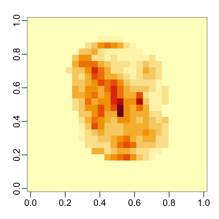
The following function computes the importance of each feature:
We can see which features are being used most by plotting an image:
32.4 Visual assessments
An important part of data analysis is visualizing results to determine why we are failing. How we do this depends on the application. Below we show the images of digits for which we made an incorrect prediction. We can compare what we get with kNN to random forest.
Here are some errors for the random forest:
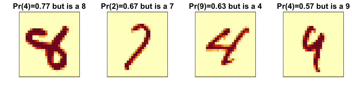
By examining errors like this we often find specific weaknesses to algorithms or parameter choices and can try to correct them.
32.5 Ensembles
The idea of an ensemble is similar to the idea of combining data from different pollsters to obtain a better estimate of the true support for each candidate.
In machine learning, one can usually greatly improve the final results by combining the results of different algorithms.
Here is a simple example where we compute new class probabilities by taking the average of random forest and kNN. We can see that the accuracy improves to 0.96:
p_rf <- predict(fit_rf, x_test[,col_index], type = "prob")
p_rf<- p_rf / rowSums(p_rf)
p_knn  <- predict(fit_knn, x_test[,col_index])
p <- (p_rf + p_knn)/2
y_pred <- factor(apply(p, 1, which.max)-1)
confusionMatrix(y_pred, y_test)$overall["Accuracy"]
#> Accuracy
#>    0.961
In the exercises we are going to build several machine learning models for the
mnist_27 dataset and then build an ensemble.
32.6 Exercises
1. Use the mnist_27 training set to build a model with several of the models available from the caret package. For example, you can try these:
models <- c("glm", "lda",  "naive_bayes",  "svmLinear", "gamboost",
            "gamLoess", "qda", "knn", "kknn", "loclda", "gam", "rf",
            "ranger","wsrf", "Rborist", "avNNet", "mlp", "monmlp", "gbm",
            "adaboost", "svmRadial", "svmRadialCost", "svmRadialSigma")
We have not explained many of these, but apply them anyway using train with all the default parameters. Keep the results in a list. You might need to install some packages. Keep in mind that you will likely get some warnings.
2. Now that you have all the trained models in a list, use sapply or map to create a matrix of predictions for the test set. You should end up with a matrix with length(mnist_27$test$y) rows and length(models) columns.
3. Now compute accuracy for each model on the test set.
4. Now build an ensemble prediction by majority vote and compute its accuracy.
5. Earlier we computed the accuracy of each method on the training set and noticed they varied. Which individual methods do better than the ensemble?
6. It is tempting to remove the methods that do not perform well and re-do the ensemble. The problem with this approach is that we are using the test data to make a decision. However, we could use the accuracy estimates obtained from cross validation with the training data. Obtain these estimates and save them in an object.
7. Now let’s only consider the methods with an estimated accuracy of 0.8 when constructing the ensemble. What is the accuracy now?
8. Advanced: If two methods give results that are the same, ensembling them will not change the results at all. For each pair of metrics compare the percent of time they call the same thing. Then use the heatmap function to visualize the results. Hint: use the method = "binary" argument in the dist function.
9. Advanced: Note that each method can also produce an estimated conditional probability. Instead of majority vote we can take the average of these estimated conditional probabilities. For most methods, we can the use the type = "prob" in the train function. However, some of the methods require you to use the argument trControl=trainControl(classProbs=TRUE) when calling train. Also these methods do not work if classes have numbers as names. Hint: change the levels like this:
dat$train$y <- recode_factor(dat$train$y, "2"="two", "7"="seven")
dat$test$y <- recode_factor(dat$test$y, "2"="two", "7"="seven")
10. In this chapter, we illustrated a couple of machine learning algorithms on a subset of the MNIST dataset. Try fitting a model to the entire dataset.