Chapter 1 Getting started with R and RStudio
1.1 Why R?
R is not a programming language like C or Java. It was not created by software engineers for software development. Instead, it was developed by statisticians as an interactive environment for data analysis. You can read the full history in the paper A Brief History of S1. The interactivity is an indispensable feature in data science because, as you will soon learn, the ability to quickly explore data is a necessity for success in this field. However, like in other programming languages, you can save your work as scripts that can be easily executed at any moment. These scripts serve as a record of the analysis you performed, a key feature that facilitates reproducible work. If you are an expert programmer, you should not expect R to follow the conventions you are used to since you will be disappointed. If you are patient, you will come to appreciate the unequal power of R when it comes to data analysis and, specifically, data visualization.
Other attractive features of R are:
- R is free and open source2.
- It runs on all major platforms: Windows, Mac Os, UNIX/Linux.
- Scripts and data objects can be shared seamlessly across platforms.
- There is a large, growing, and active community of R users and, as a result, there are numerous resources for learning and asking questions3 4 5.
- It is easy for others to contribute add-ons which enables developers to share software implementations of new data science methodologies. This gives R users early access to the latest methods and to tools which are developed for a wide variety of disciplines, including ecology, molecular biology, social sciences, and geography, just to name a few examples.
1.2 The R console
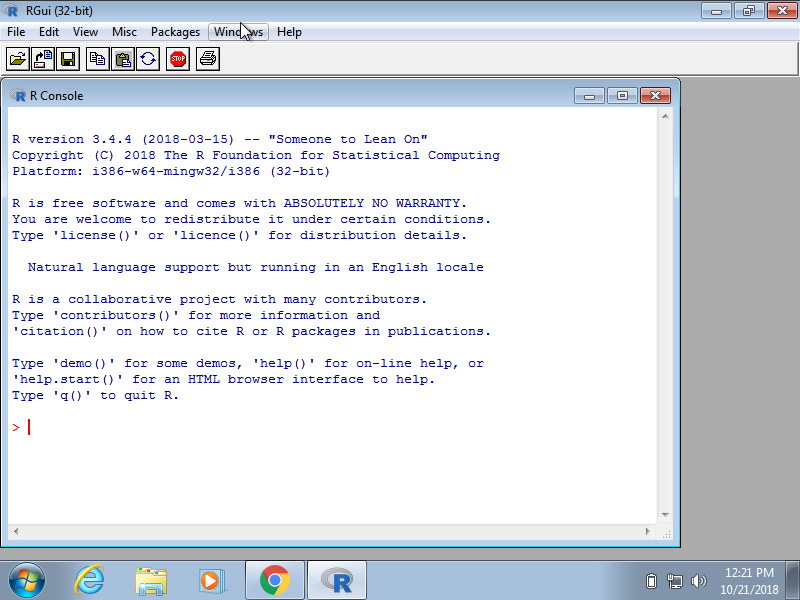
Interactive data analysis usually occurs on the R console that executes commands as you type them. There are several ways to gain access to an R console. One way is to simply start R on your computer. The console looks something like this:
As a quick example, try using the console to calculate a 15% tip on a meal that cost $19.71:
Note that in this book, grey boxes are used to show R code typed into the R console. The symbol #> is used to denote what the R console outputs.
1.3 Scripts
One of the great advantages of R over point-and-click analysis software is that you can save your work as scripts. You can edit and save these scripts using a text editor. The material in this book was developed using the interactive integrated development environment (IDE) RStudio6. RStudio includes an editor with many R specific features, a console to execute your code, and other useful panes, including one to show figures.
Most web-based R consoles also provide a pane to edit scripts, but not all permit you to save the scripts for later use.
All the R scripts used to generate this book can be found on GitHub7.
1.4 RStudio
RStudio will be our launching pad for data science projects. It not only provides an editor for us to create and edit our scripts but also provides many other useful tools. In this section, we go over some of the basics.
1.4.1 The panes
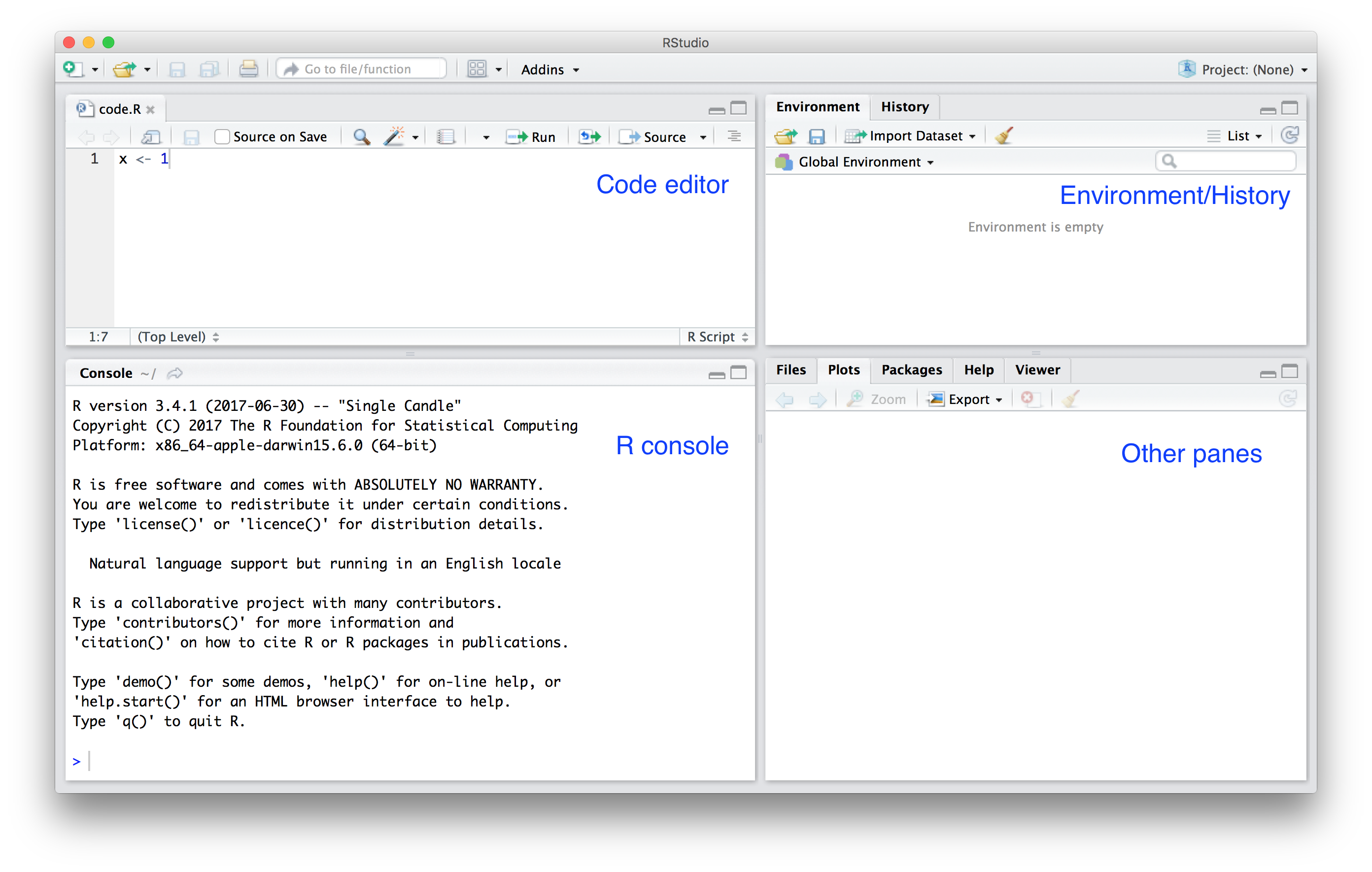
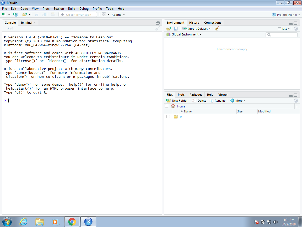
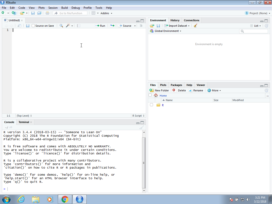
When you start RStudio for the first time, you will see three panes. The left pane shows the R console. On the right, the top pane includes tabs such as Environment and History, while the bottom pane shows five tabs: File, Plots, Packages, Help, and Viewer (these tabs may change in new versions). You can click on each tab to move across the different features.
To start a new script, you can click on File, then New File, then R Script.
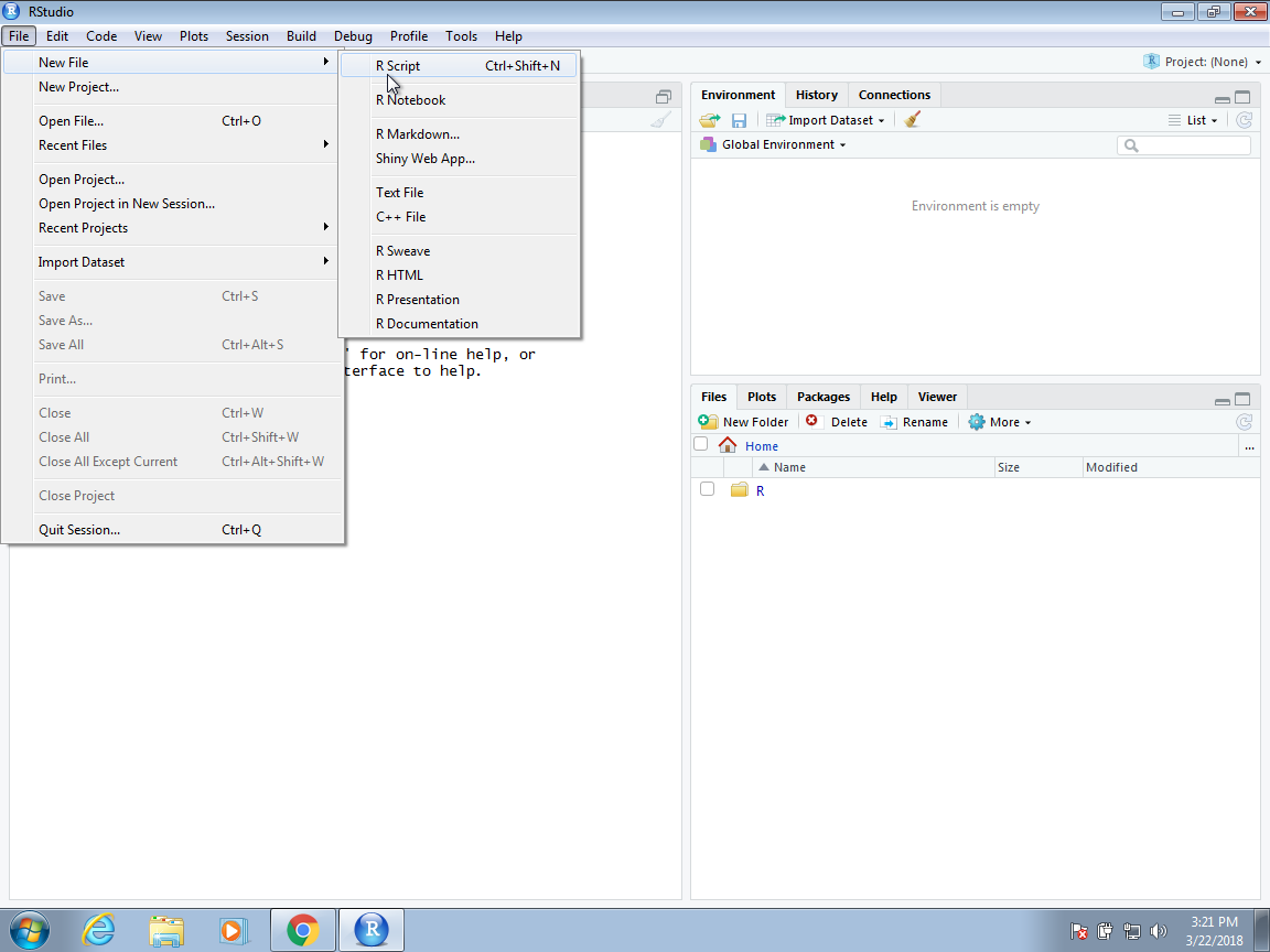
This starts a new pane on the left and it is here where you can start writing your script.
1.4.2 Key bindings
Many tasks we perform with the mouse can be achieved with a combination of key strokes instead. These keyboard versions for performing tasks are referred to as key bindings. For example, we just showed how to use the mouse to start a new script, but you can also use a key binding: Ctrl+Shift+N on Windows and command+shift+N on the Mac.
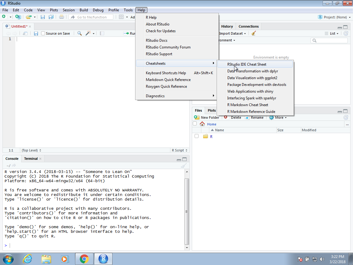
Although in this tutorial we often show how to use the mouse, we highly recommend that you memorize key bindings for the operations you use most. RStudio provides a useful cheat sheet with the most widely used commands. You can get it from RStudio directly:
You might want to keep this handy so you can look up key-bindings when you find yourself performing repetitive point-and-clicking.
1.4.3 Running commands while editing scripts
There are many editors specifically made for coding. These are useful because color and indentation are automatically added to make code more readable. RStudio is one of these editors, and it was specifically developed for R. One of the main advantages provided by RStudio over other editors is that we can test our code easily as we edit our scripts. Below we show an example.
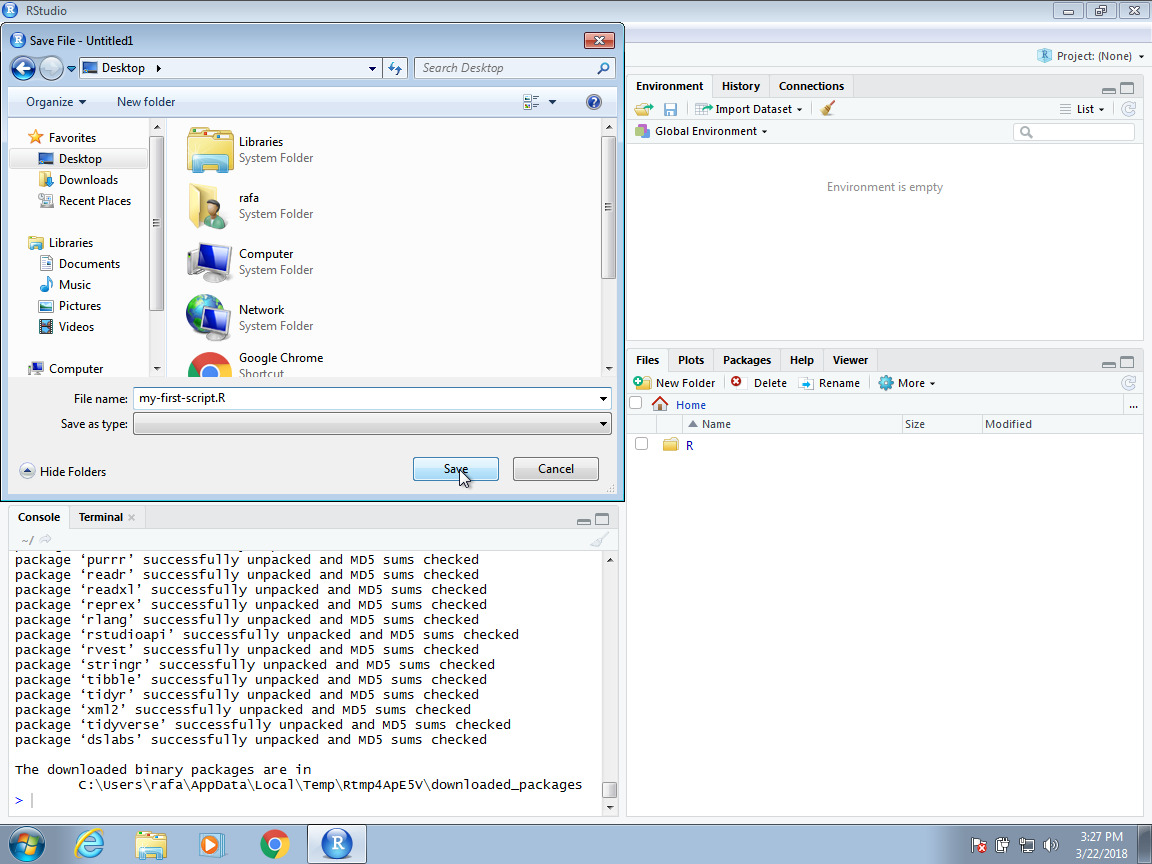
Let’s start by opening a new script as we did before. A next step is to give the script a name. We can do this through the editor by saving the current new unnamed script. To do this, click on the save icon or use the key binding Ctrl+S on Windows and command+S on the Mac.
When you ask for the document to be saved for the first time, RStudio will prompt you for a name. A good convention is to use a descriptive name, with lower case letters, no spaces, only hyphens to separate words, and then followed by the suffix .R. We will call this script my-first-script.R.
Now we are ready to start editing our first script. The first lines of code in an R script are dedicated to loading the libraries we will use. Another useful RStudio feature is that once we type library() it starts auto-completing with libraries that we have installed. Note what happens when we type library(ti):
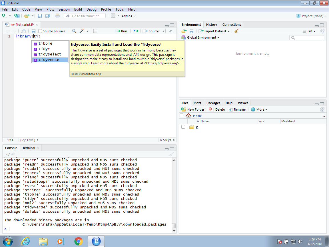
Another feature you may have noticed is that when you type library( the second parenthesis is automatically added. This will help you avoid one of the most common errors in coding: forgetting to close a parenthesis.
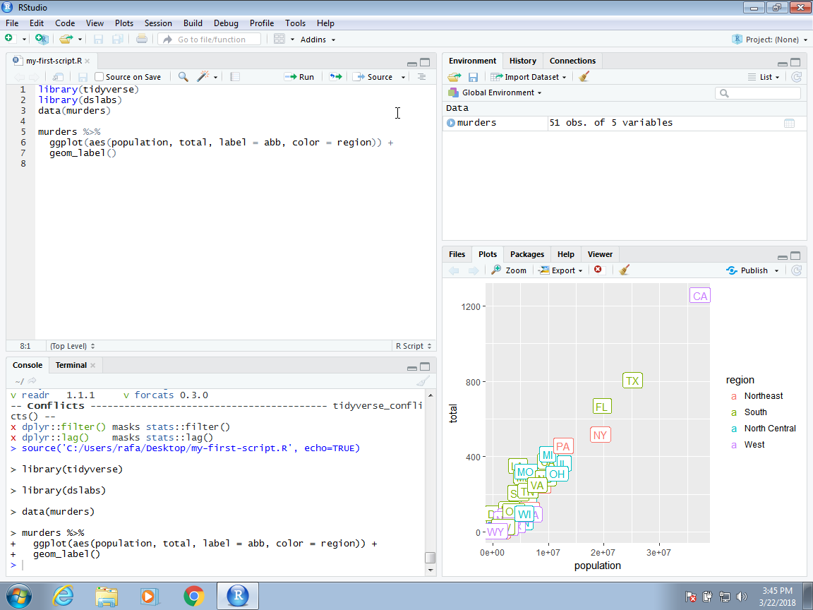
Now we can continue to write code. As an example, we will make a graph showing murder totals versus population totals by state. Once you are done writing the code needed to make this plot, you can try it out by executing the code. To do this, click on the Run button on the upper right side of the editing pane. You can also use the key binding: Ctrl+Shift+Enter on Windows or command+shift+return on the Mac.
Once you run the code, you will see it appear in the R console and, in this case, the generated plot appears in the plots console. Note that the plot console has a useful interface that permits you to click back and forward across different plots, zoom in to the plot, or save the plots as files.
To run one line at a time instead of the entire script, you can use Control-Enter on Windows and command-return on the Mac.
1.4.4 Changing global options
You can change the look and functionality of RStudio quite a bit.
To change the global options you click on Tools then Global Options….
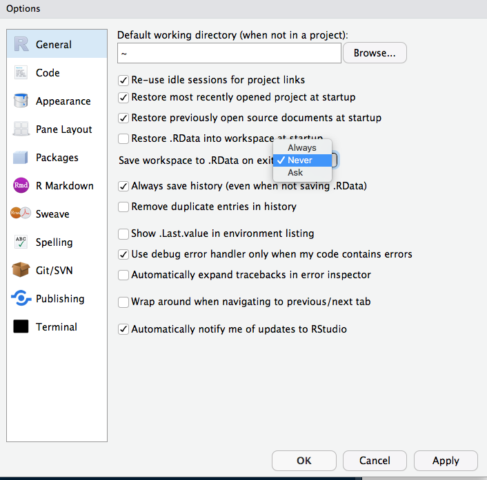
As an example we show how to make a change that we highly recommend. This is to change the Save workspace to .RData on exit to Never and uncheck the Restore .RData into workspace at start. By default, when you exit R saves all the objects you have created into a file called .RData. This is done so that when you restart the session in the same folder, it will load these objects. We find that this causes confusion especially when we share code with colleagues and assume they have this .RData file. To change these options, make your General settings look like this:
1.5 Installing R packages
The functionality provided by a fresh install of R is only a small fraction of what is possible. In fact, we refer to what you get after your first install as base R. The extra functionality comes from add-ons available from developers. There are currently hundreds of these available from CRAN and many others shared via other repositories such as GitHub. However, because not everybody needs all available functionality, R instead makes different components available via packages. R makes it very easy to install packages from within R. For example, to install the dslabs package, which we use to share datasets and code related to this book, you would type:
In RStudio, you can navigate to the Tools tab and select install packages. We can then load the package into our R sessions using the library function:
As you go through this book, you will see that we load packages without installing them. This is because once you install a package, it remains installed and only needs to be loaded with library. The package remains loaded until we quit the R session. If you try to load a package and get an error, it probably means you need to
install it first.
We can install more than one package at once by feeding a character vector to this function:
Note that installing tidyverse actually installs several packages. This commonly occurs when a package has dependencies, or uses functions from other packages. When you load a package using library, you also load its dependencies.
Once packages are installed, you can load them into R and you do not need to install them again, unless you install a fresh version of R. Remember packages are installed in R not RStudio.
It is helpful to keep a list of all the packages you need for your work in a script because if you need to perform a fresh install of R, you can re-install all your packages by simply running a script.
You can see all the packages you have installed using the following function: